Example scripts
Copy-paste the text blocks below and save them as .py files to try them out.
Ground state volume of bcc bulk iron
#!/usr/bin/python

# An example script of how to automatically
# calculate the equilibrium volume and
# bulk modulus of bulk bcc Fe using pyEMTO.

import pyemto

emtopath = "/wrk/hpleva/pyEMTO_examples/fe" # Define a folder for our KGRN and KFCD input and output files.
latpath  = "/wrk/hpleva/structures"         # Define a folder where the BMDL, KSTR and KFCD input and output files
                                            # will be located.

fe = pyemto.System(folder=emtopath)  # Create a new instance of the pyemto System-class.

# Let's calculate the equilibrium volume and bulk modulus of Fe.

# Initialize the system using the bulk.() function:

fe.bulk(lat     = 'bcc',   # We want to use the bcc structure.
        latpath = latpath, # Path to the folder where the structure files are located.
        afm     = 'F',     # We want to do a ferromagnetic calculation.
        atoms   = ['Fe'],  # A list of atoms.
        splts   = [2.0],   # A list of magnetic splittings.
        expan   = 'M',     # We want to use the double-Taylor expansion.
        sofc    = 'Y',     # We want to use soft-core approximation.
        xc      = 'PBE',   # We want to use the PBE functional.
        amix    = 0.05,    # Density mixing.
        nky     = 21)      # Number of k-points.

sws = [2.6,2.62,2.64,2.66,2.68,2.70] # A list of Wigner-Seitz radii

# Generate all the necessary input files with this function:
#fe.lattice_constants_batch_generate(sws=sws)

#The newly created batch scripts are then submitted by hand.

# Analyze the results using this function once all the calculations
# have finished:
#fe.lattice_constants_analyze(sws=sws)

# This function combines the features of the previous two:
fe.lattice_constants_batch_calculate(sws=sws)
The output of this script should look like this:
Submitted batch job 1021841
Submitted batch job 1021842
Submitted batch job 1021843
Submitted batch job 1021844
Submitted batch job 1021845
Submitted batch job 1021846

wait_for_jobs: Submitted 6 jobs
wait_for_jobs: Will be requesting job statuses every 60 seconds

0:01:00 {'RUNNING': 6} (  0% completion)
0:02:00 {'RUNNING': 6} (  0% completion)
0:03:00 {'RUNNING': 6} (  0% completion)
0:04:00 {'COMPLETED': 4, 'RUNNING': 2} ( 66% completion)
0:05:00 {'COMPLETED': 6} (100% completion)
completed 6 batch jobs in 0:05:00

*****lattice_constants_analyze*****


********************************
lattice_constants_analyze(cubic)
********************************
  SWS        Energy
2.600000  -2545.605517
2.620000  -2545.606394
2.640000  -2545.606680
2.660000  -2545.606435
2.680000  -2545.605705
2.700000  -2545.604616


5.2.2015 -- 16:21:13
JOBNAM = fe1.00 -- PBE

Using morse function

Chi squared         = 2.7459052408e-10
Reduced Chi squared = 1.3729526204e-10
R squared           = 0.999907593903

morse parameters:

a      =     0.117551
b      =  -122.663728
c      = 32000.491593
lambda =     2.370150

Ground state parameters:

V0           =     2.640005 Bohr^3 (unit cell volume)
             =     2.640005 Bohr   (WS-radius)
E0           = -2545.606678 Ry
Bmod         =   195.204183 GPa
Grun. param. =     3.128604

sws            Einp           Eout          Residual       err (% * 10**6)
2.600000  -2545.605517  -2545.605515      0.000002       -0.000870
2.620000  -2545.606394  -2545.606400     -0.000006        0.002524
2.640000  -2545.606680  -2545.606678      0.000002       -0.000950
2.660000  -2545.606435  -2545.606426      0.000009       -0.003632
2.680000  -2545.605705  -2545.605716     -0.000011        0.004368
2.700000  -2545.604616  -2545.604612      0.000004       -0.001440


lattice_constants_analyze(cubic):
sws0 =      2.640005
B0   =    195.204183
E0   =  -2545.606678
Elastic constants of bcc bulk iron
#!/usr/bin/python

# An example script showing how to automatically calculate
# the elastic constants of bulk bcc Fe using pyEMTO.

import pyemto

emtopath = "/wrk/hpleva/pyEMTO_examples/fe_elastic_constants" # Define a folder for our KGRN and KFCD input and output files.
latpath  = "/wrk/hpleva/structures"                           # Define a folder where the BMDL, KSTR and KFCD input and output files
                                                              # will be located.

fe = pyemto.System(folder=emtopath)  # Create a new instance of the pyemto System-class.

# Let's calculate the elastic constants of Fe.

fe.bulk(lat     = 'bcc',   # We want to use the bcc structure.
        latpath = latpath, # Path to the folder where the structure files are located.
        afm     = 'F',     # We want to do a ferromagnetic calculation.
        atoms   = ['Fe'],  # A list of atoms.
        splts   = [2.0],   # A list of magnetic splittings.
        expan   = 'M',     # We want to use the double-Taylor expansion.
        sofc    = 'Y',     # We want to use soft-core approximation.
        xc      = 'PBE',   # We want to use the PBE functional.
        amix    = 0.05)    # Mixing parameter.

sws0 = 2.64 # Eq. WS-radius that we computed previously.
B0   = 195  # Eq. bulk modulus.

# Generate all the necessary input files with this function:
#fe.elastic_constants_batch_generate(sws=sws0)

#The newly created batch scripts are then submitted by hand.

# Analyze the results using this function once all the calculations
# have finished:
#fe.elastic_constants_analyze(sws=sws,bmod=B0)

# This function combines the features of the previous two:
fe.elastic_constants_batch_calculate(sws=sws0,bmod=B0)
The output of this script should look like this:
Submitted batch job 1021848
Submitted batch job 1021849
Submitted batch job 1021850
Submitted batch job 1021851
Submitted batch job 1021852
Submitted batch job 1021853
Submitted batch job 1021854
Submitted batch job 1021855
Submitted batch job 1021856
Submitted batch job 1021857
Submitted batch job 1021858
Submitted batch job 1021859

wait_for_jobs: Submitted 12 jobs
wait_for_jobs: Will be requesting job statuses every 60 seconds

0:01:00 {'RUNNING': 12} (  0% completion)
0:02:00 {'RUNNING': 12} (  0% completion)
0:03:00 {'RUNNING': 12} (  0% completion)
0:04:00 {'RUNNING': 12} (  0% completion)
0:05:00 {'RUNNING': 12} (  0% completion)
0:06:00 {'RUNNING': 12} (  0% completion)
0:07:00 {'RUNNING': 12} (  0% completion)
0:08:01 {'RUNNING': 12} (  0% completion)
0:09:01 {'RUNNING': 12} (  0% completion)
0:10:01 {'RUNNING': 12} (  0% completion)
0:11:01 {'RUNNING': 12} (  0% completion)
0:12:01 {'RUNNING': 12} (  0% completion)
0:13:01 {'RUNNING': 12} (  0% completion)
0:14:01 {'RUNNING': 12} (  0% completion)
0:15:01 {'RUNNING': 12} (  0% completion)
0:16:01 {'RUNNING': 12} (  0% completion)
0:17:02 {'RUNNING': 12} (  0% completion)
0:18:02 {'RUNNING': 12} (  0% completion)
0:19:02 {'RUNNING': 12} (  0% completion)
0:20:02 {'RUNNING': 12} (  0% completion)
0:21:02 {'RUNNING': 12} (  0% completion)
0:22:02 {'RUNNING': 12} (  0% completion)
0:23:02 {'RUNNING': 12} (  0% completion)
0:24:02 {'RUNNING': 12} (  0% completion)
0:25:03 {'RUNNING': 12} (  0% completion)
0:26:03 {'RUNNING': 12} (  0% completion)
0:27:03 {'RUNNING': 12} (  0% completion)
0:28:03 {'RUNNING': 12} (  0% completion)
0:29:03 {'RUNNING': 12} (  0% completion)
0:30:03 {'RUNNING': 12} (  0% completion)
0:31:03 {'RUNNING': 12} (  0% completion)
0:32:03 {'RUNNING': 12} (  0% completion)
0:33:03 {'RUNNING': 12} (  0% completion)
0:34:04 {'RUNNING': 12} (  0% completion)
0:35:04 {'RUNNING': 12} (  0% completion)
0:36:04 {'RUNNING': 12} (  0% completion)
0:37:04 {'RUNNING': 12} (  0% completion)
0:38:04 {'RUNNING': 12} (  0% completion)
0:39:04 {'RUNNING': 12} (  0% completion)
0:40:04 {'RUNNING': 12} (  0% completion)
0:41:04 {'RUNNING': 12} (  0% completion)
0:42:05 {'RUNNING': 12} (  0% completion)
0:43:05 {'RUNNING': 12} (  0% completion)
0:44:05 {'RUNNING': 12} (  0% completion)
0:45:05 {'RUNNING': 12} (  0% completion)
0:46:05 {'RUNNING': 12} (  0% completion)
0:47:05 {'RUNNING': 12} (  0% completion)
0:48:05 {'RUNNING': 12} (  0% completion)
0:49:05 {'RUNNING': 12} (  0% completion)
0:50:05 {'RUNNING': 12} (  0% completion)
0:51:06 {'RUNNING': 12} (  0% completion)
0:52:06 {'RUNNING': 12} (  0% completion)
0:53:06 {'RUNNING': 12} (  0% completion)
0:54:06 {'RUNNING': 12} (  0% completion)
0:55:06 {'RUNNING': 12} (  0% completion)
0:56:06 {'RUNNING': 12} (  0% completion)
0:57:06 {'RUNNING': 12} (  0% completion)
0:58:06 {'RUNNING': 12} (  0% completion)
0:59:07 {'RUNNING': 11, 'COMPLETED': 1} (  8% completion)
1:00:07 {'RUNNING': 10, 'COMPLETED': 2} ( 16% completion)
1:01:07 {'RUNNING': 9, 'COMPLETED': 3} ( 25% completion)
1:02:07 {'RUNNING': 9, 'COMPLETED': 3} ( 25% completion)
1:03:07 {'RUNNING': 9, 'COMPLETED': 3} ( 25% completion)
1:04:07 {'RUNNING': 9, 'COMPLETED': 3} ( 25% completion)
1:05:07 {'RUNNING': 9, 'COMPLETED': 3} ( 25% completion)
1:06:07 {'RUNNING': 9, 'COMPLETED': 3} ( 25% completion)
1:07:08 {'RUNNING': 9, 'COMPLETED': 3} ( 25% completion)
1:08:08 {'RUNNING': 8, 'COMPLETED': 4} ( 33% completion)
1:09:08 {'COMPLETED': 6, 'RUNNING': 6} ( 50% completion)
1:10:08 {'COMPLETED': 6, 'RUNNING': 6} ( 50% completion)
1:11:08 {'COMPLETED': 6, 'RUNNING': 6} ( 50% completion)
1:12:08 {'COMPLETED': 6, 'RUNNING': 6} ( 50% completion)
1:13:08 {'COMPLETED': 6, 'RUNNING': 6} ( 50% completion)
1:14:08 {'COMPLETED': 6, 'RUNNING': 6} ( 50% completion)
1:15:09 {'COMPLETED': 6, 'RUNNING': 6} ( 50% completion)
1:16:09 {'COMPLETED': 6, 'RUNNING': 6} ( 50% completion)
1:17:09 {'COMPLETED': 6, 'RUNNING': 6} ( 50% completion)
1:18:09 {'COMPLETED': 6, 'RUNNING': 6} ( 50% completion)
1:19:09 {'COMPLETED': 7, 'RUNNING': 5} ( 58% completion)
1:20:09 {'COMPLETED': 7, 'RUNNING': 5} ( 58% completion)
1:21:09 {'COMPLETED': 8, 'RUNNING': 4} ( 66% completion)
1:22:09 {'COMPLETED': 10, 'RUNNING': 2} ( 83% completion)
1:23:10 {'COMPLETED': 10, 'RUNNING': 2} ( 83% completion)
1:24:10 {'COMPLETED': 10, 'RUNNING': 2} ( 83% completion)
1:25:10 {'COMPLETED': 11, 'RUNNING': 1} ( 91% completion)
1:26:10 {'COMPLETED': 12} (100% completion)
completed 12 batch jobs in 1:26:10

***cubic_elastic_constants***

fe1.00

c11(GPa) = 299.60
c12(GPa) = 142.70
c44(GPa) = 105.95
c' (GPa) =  78.45
B  (GPa) = 195.00

Voigt average:

BV(GPa)  = 195.00
GV(GPa)  =  94.95
EV(GPa)  = 245.07
vV(GPa)  =   0.29

Reuss average:

BR(GPa)  = 195.00
GR(GPa)  =  92.92
ER(GPa)  = 240.55
vR(GPa)  =   0.29

Hill average:

BH(GPa)  = 195.00
GH(GPa)  =  93.93
EH(GPa)  = 242.81
vH(GPa)  =   0.29

Elastic anisotropy:

AVR(GPa)  =   0.01
Ground state volume and elastic constants of hcp bulk titanium
#!/usr/bin/python

# This script will automatically accomplish:

#  1. Calculate the equilibrium volume and bulk modulus of hcp Ti.
#  2. Calculate the elastic constants of hcp Ti.

import pyemto
import os
import numpy as np

# It is recommended to always use absolute paths
folder = os.getcwd()                # Get current working directory.
latpath = "/wrk/hpleva/structures"  # Folder where the structure files are located.
emtopath = folder+"/ti_hcp"         # Folder where the calculation take place.

ti_hcp=pyemto.System(folder=emtopath)

# Initialize the bulk system using the bulk() function:
ti_hcp.bulk(lat='hcp',
            latpath=latpath,
            atoms=['Ti'],
            sws=3.0,
            amix=0.02,
            efmix=0.9,
            expan='M',
            sofc='Y',
            xc='P07',           # Use PBEsol
            nky=31,             # k-points
            nkz=19,             # k-points
            runtime='24:00:00') # Allow large enough timelimit for SLURM

sws = np.linspace(2.9,3.1,7) # A list of 7 different volumes from 2.9 to 3.1


sws0,ca0,B0,e0,R0,cs0 = ti_hcp.lattice_constants_batch_calculate(sws=sws)
ti_hcp.elastic_constants_batch_calculate(sws=sws0,bmod=B0,ca=ca0,R=R0,cs=cs0)

# If the batch jobs are submitted by hand use these functions.

# To evaluate the results, comment out the _generate functions
# and uncomment the _analyze functions.

ti_hcp.lattice_constants_batch_generate(sws=sws)
#ti_hcp.lattice_constants_analyze(sws=sws)

# Results. These are inputed to the elastic_constants functions.
#sws0 =      3.002260
#ca0  =      1.610122
#B0   =    115.952318
#E0   =  -1705.738844
#R0   =      0.019532
#cs0  =    498.360422

#ti_hcp.elastic_constants_batch_generate(sws=sws0,ca=ca0)
#ti_hcp.elastic_constants_analyze(sws=sws0,bmod=B0,ca=ca0,R=R0,cs=cs0)
The output of this script should look like this:
Submitted batch job 1021973
Submitted batch job 1021974
Submitted batch job 1021975
Submitted batch job 1021976
Submitted batch job 1021977
Submitted batch job 1021978
Submitted batch job 1021979
Submitted batch job 1021980
Submitted batch job 1021981
Submitted batch job 1021982
Submitted batch job 1021983
Submitted batch job 1021984
Submitted batch job 1021985
Submitted batch job 1021986
Submitted batch job 1021987
Submitted batch job 1021988
Submitted batch job 1021989
Submitted batch job 1021990
Submitted batch job 1021991
Submitted batch job 1021992
Submitted batch job 1021993
Submitted batch job 1021994
Submitted batch job 1021995
Submitted batch job 1021996
Submitted batch job 1021997
Submitted batch job 1021998
Submitted batch job 1021999
Submitted batch job 1022000
Submitted batch job 1022001
Submitted batch job 1022002
Submitted batch job 1022003
Submitted batch job 1022004
Submitted batch job 1022005
Submitted batch job 1022006
Submitted batch job 1022007
Submitted batch job 1022008
Submitted batch job 1022009
Submitted batch job 1022010
Submitted batch job 1022011
Submitted batch job 1022012
Submitted batch job 1022013
Submitted batch job 1022014
Submitted batch job 1022015
Submitted batch job 1022016
Submitted batch job 1022017
Submitted batch job 1022018
Submitted batch job 1022019
Submitted batch job 1022020
Submitted batch job 1022021
()
wait_for_jobs: Submitted 49 jobs
wait_for_jobs: Will be requesting job statuses every 60 seconds

0:01:00 {'RUNNING': 49} (  0% completion)
0:02:00 {'RUNNING': 49} (  0% completion)
0:03:00 {'RUNNING': 49} (  0% completion)
0:04:00 {'RUNNING': 49} (  0% completion)
0:05:01 {'RUNNING': 49} (  0% completion)
0:06:01 {'RUNNING': 49} (  0% completion)
0:07:01 {'RUNNING': 49} (  0% completion)
0:08:01 {'RUNNING': 49} (  0% completion)
0:09:02 {'RUNNING': 49} (  0% completion)
0:10:02 {'RUNNING': 49} (  0% completion)
0:11:02 {'RUNNING': 49} (  0% completion)
0:12:02 {'RUNNING': 49} (  0% completion)
0:13:02 {'RUNNING': 49} (  0% completion)
0:14:02 {'RUNNING': 49} (  0% completion)
0:15:02 {'RUNNING': 49} (  0% completion)
0:16:03 {'RUNNING': 49} (  0% completion)
0:17:03 {'RUNNING': 49} (  0% completion)
0:18:03 {'RUNNING': 49} (  0% completion)
0:19:03 {'RUNNING': 49} (  0% completion)
0:20:03 {'RUNNING': 49} (  0% completion)
0:21:03 {'RUNNING': 49} (  0% completion)
0:22:03 {'RUNNING': 49} (  0% completion)
0:23:03 {'RUNNING': 49} (  0% completion)
0:24:04 {'RUNNING': 49} (  0% completion)
0:25:04 {'RUNNING': 49} (  0% completion)
0:26:04 {'RUNNING': 48, 'COMPLETED': 1} (  2% completion)
0:27:04 {'RUNNING': 47, 'COMPLETED': 2} (  4% completion)
0:28:04 {'RUNNING': 46, 'COMPLETED': 3} (  6% completion)
0:29:04 {'RUNNING': 42, 'COMPLETED': 7} ( 14% completion)
0:30:04 {'RUNNING': 40, 'COMPLETED': 9} ( 18% completion)
0:31:05 {'COMPLETED': 12, 'RUNNING': 37} ( 24% completion)
0:32:05 {'COMPLETED': 15, 'RUNNING': 34} ( 30% completion)
0:33:05 {'COMPLETED': 15, 'RUNNING': 34} ( 30% completion)
0:34:05 {'COMPLETED': 15, 'RUNNING': 34} ( 30% completion)
0:35:05 {'COMPLETED': 18, 'RUNNING': 31} ( 36% completion)
0:36:05 {'COMPLETED': 29, 'RUNNING': 20} ( 59% completion)
0:37:05 {'COMPLETED': 44, 'RUNNING': 5} ( 89% completion)
0:38:06 {'COMPLETED': 49} (100% completion)
completed 49 batch jobs in 0:38:06

*****lattice_constants_analyze*****


******************************
lattice_constants_analyze(hcp)
******************************
  SWS        Energy0        c'a0
2.900000  -1705.733796  1.613939
2.933333  -1705.736608  1.612527
2.966667  -1705.738262  1.611196
3.000000  -1705.738843  1.610175
3.033333  -1705.738424  1.609326
3.066667  -1705.737080  1.608336
3.100000  -1705.734889  1.607505


5.2.2015 -- 18:51:51
JOBNAM = ti1.00 -- P07

Using morse function

Chi squared         = 1.16375610448e-11
Reduced Chi squared = 3.87918701493e-12
R squared           = 0.999999464309

morse parameters:

a      =     0.757678
b      =   -15.168890
c      =    75.921091
lambda =     0.767287

Ground state parameters:

V0           =     3.002260 Bohr^3 (unit cell volume)
             =     3.002260 Bohr   (WS-radius)
E0           = -1705.738844 Ry
Bmod         =   115.952318 GPa
Grun. param. =     1.151798

sws            Einp           Eout          Residual       err (% * 10**6)
2.900000  -1705.733796  -1705.733796      0.000000       -0.000275
2.933333  -1705.736608  -1705.736609     -0.000001        0.000498
2.966667  -1705.738262  -1705.738263     -0.000001        0.000376
3.000000  -1705.738843  -1705.738842      0.000001       -0.000810
3.033333  -1705.738424  -1705.738423      0.000001       -0.000680
3.066667  -1705.737080  -1705.737082     -0.000002        0.001450
3.100000  -1705.734889  -1705.734889      0.000001       -0.000558


5.2.2015 -- 18:51:51
JOBNAM = ti1.00 -- P07

Using morse function

Chi squared         = 1.06749728331e-10
Reduced Chi squared = 3.5583242777e-11
R squared           = 0.999995355882

morse parameters:

a      =     0.748045
b      =   -15.100334
c      =    76.203651
lambda =     0.769114

Ground state parameters:

V0           =     3.005849 Bohr^3 (unit cell volume)
             =     3.005849 Bohr   (WS-radius)
E0           = -1705.736830 Ry
Bmod         =   114.888885 GPa
Grun. param. =     1.155920

sws            Einp           Eout          Residual       err (% * 10**6)
2.900000  -1705.731449  -1705.731449     -0.000000        0.000021
2.933333  -1705.734368  -1705.734369     -0.000001        0.000770
2.966667  -1705.736134  -1705.736130      0.000004       -0.002260
3.000000  -1705.736814  -1705.736815     -0.000001        0.000665
3.033333  -1705.736497  -1705.736503     -0.000006        0.003550
3.066667  -1705.735275  -1705.735268      0.000007       -0.004035
3.100000  -1705.733178  -1705.733180     -0.000002        0.001288


5.2.2015 -- 18:51:51
JOBNAM = ti1.00 -- P07

Using morse function

Chi squared         = 3.64530335255e-11
Reduced Chi squared = 1.21510111752e-11
R squared           = 0.999998386204

morse parameters:

a      =     0.743238
b      =   -15.271044
c      =    78.441514
lambda =     0.775451

Ground state parameters:

V0           =     3.004114 Bohr^3 (unit cell volume)
             =     3.004114 Bohr   (WS-radius)
E0           = -1705.737897 Ry
Bmod         =   116.104730 GPa
Grun. param. =     1.164771

sws            Einp           Eout          Residual       err (% * 10**6)
2.900000  -1705.732644  -1705.732643      0.000001       -0.000875
2.933333  -1705.735527  -1705.735531     -0.000004        0.002534
2.966667  -1705.737255  -1705.737252      0.000003       -0.001704
3.000000  -1705.737891  -1705.737890      0.000001       -0.000729
3.033333  -1705.737524  -1705.737524     -0.000000        0.000183
3.066667  -1705.736229  -1705.736231     -0.000002        0.001216
3.100000  -1705.734082  -1705.734081      0.000001       -0.000625


5.2.2015 -- 18:51:51
JOBNAM = ti1.00 -- P07

Using morse function

Chi squared         = 1.18175890217e-11
Reduced Chi squared = 3.93919634056e-12
R squared           = 0.999999463488

morse parameters:

a      =     0.759517
b      =   -15.168958
c      =    75.737639
lambda =     0.766269

Ground state parameters:

V0           =     3.003084 Bohr^3 (unit cell volume)
             =     3.003084 Bohr   (WS-radius)
E0           = -1705.738555 Ry
Bmod         =   115.894284 GPa
Grun. param. =     1.150586

sws            Einp           Eout          Residual       err (% * 10**6)
2.900000  -1705.733423  -1705.733423     -0.000000        0.000259
2.933333  -1705.736267  -1705.736265      0.000002       -0.001035
2.966667  -1705.737944  -1705.737946     -0.000002        0.001386
3.000000  -1705.738551  -1705.738550      0.000001       -0.000391
3.033333  -1705.738157  -1705.738156      0.000001       -0.000679
3.066667  -1705.736836  -1705.736837     -0.000001        0.000606
3.100000  -1705.734664  -1705.734664      0.000000       -0.000147


5.2.2015 -- 18:51:51
JOBNAM = ti1.00 -- P07

Using morse function

Chi squared         = 5.45131762039e-12
Reduced Chi squared = 1.81710587346e-12
R squared           = 0.999999749818

morse parameters:

a      =     0.772765
b      =   -15.129144
c      =    74.049208
lambda =     0.759794

Ground state parameters:

V0           =     3.002465 Bohr^3 (unit cell volume)
             =     3.002465 Bohr   (WS-radius)
E0           = -1705.738834 Ry
Bmod         =   115.954728 GPa
Grun. param. =     1.140627

sws            Einp           Eout          Residual       err (% * 10**6)
2.900000  -1705.733769  -1705.733768      0.000001       -0.000320
2.933333  -1705.736585  -1705.736586     -0.000001        0.000827
2.966667  -1705.738247  -1705.738246      0.000001       -0.000325
3.000000  -1705.738832  -1705.738831      0.000001       -0.000454
3.033333  -1705.738419  -1705.738419      0.000000       -0.000175
3.066667  -1705.737081  -1705.737082     -0.000001        0.000791
3.100000  -1705.734892  -1705.734891      0.000001       -0.000345


5.2.2015 -- 18:51:52
JOBNAM = ti1.00 -- P07

Using morse function

Chi squared         = 1.19109949001e-11
Reduced Chi squared = 3.97033163337e-12
R squared           = 0.999999449336

morse parameters:

a      =     0.745414
b      =   -15.182081
c      =    77.304565
lambda =     0.773045

Ground state parameters:

V0           =     3.002133 Bohr^3 (unit cell volume)
             =     3.002133 Bohr   (WS-radius)
E0           = -1705.738728 Ry
Bmod         =   115.798751 GPa
Grun. param. =     1.160392

sws            Einp           Eout          Residual       err (% * 10**6)
2.900000  -1705.733697  -1705.733697      0.000000       -0.000064
2.933333  -1705.736504  -1705.736504      0.000000       -0.000199
2.966667  -1705.738150  -1705.738152     -0.000002        0.001152
3.000000  -1705.738728  -1705.738726      0.000002       -0.001245
3.033333  -1705.738305  -1705.738305      0.000000       -0.000241
3.066667  -1705.736961  -1705.736963     -0.000002        0.000983
3.100000  -1705.734771  -1705.734770      0.000001       -0.000387


5.2.2015 -- 18:51:52
JOBNAM = ti1.00 -- P07

Using morse function

Chi squared         = 1.38286217253e-11
Reduced Chi squared = 4.60954057509e-12
R squared           = 0.999999356009

morse parameters:

a      =     0.759904
b      =   -15.070597
c      =    74.720674
lambda =     0.764158

Ground state parameters:

V0           =     3.002206 Bohr^3 (unit cell volume)
             =     3.002206 Bohr   (WS-radius)
E0           = -1705.738293 Ry
Bmod         =   115.348605 GPa
Grun. param. =     1.147079

sws            Einp           Eout          Residual       err (% * 10**6)
2.900000  -1705.733279  -1705.733278      0.000001       -0.000462
2.933333  -1705.736071  -1705.736073     -0.000002        0.001462
2.966667  -1705.737719  -1705.737717      0.000002       -0.001374
3.000000  -1705.738290  -1705.738290     -0.000000        0.000238
3.033333  -1705.737873  -1705.737873      0.000000       -0.000175
3.066667  -1705.736536  -1705.736537     -0.000001        0.000590
3.100000  -1705.734353  -1705.734353      0.000000       -0.000280


5.2.2015 -- 18:51:52
JOBNAM = ti1.00 -- P07

Using morse function

Chi squared         = 2.17769833254e-11
Reduced Chi squared = 7.25899444181e-12
R squared           = 0.99999898819

morse parameters:

a      =     0.831171
b      =   -14.866360
c      =    66.474685
lambda =     0.729592

Ground state parameters:

V0           =     3.002865 Bohr^3 (unit cell volume)
             =     3.002865 Bohr   (WS-radius)
E0           = -1705.737540 Ry
Bmod         =   114.985899 GPa
Grun. param. =     1.095434

sws            Einp           Eout          Residual       err (% * 10**6)
2.900000  -1705.732490  -1705.732491     -0.000001        0.000576
2.933333  -1705.735292  -1705.735289      0.000003       -0.001807
2.966667  -1705.736942  -1705.736944     -0.000002        0.001443
3.000000  -1705.737535  -1705.737536     -0.000001        0.000646
3.033333  -1705.737140  -1705.737138      0.000002       -0.001159
3.066667  -1705.735820  -1705.735820     -0.000000        0.000187
3.100000  -1705.733649  -1705.733649     -0.000000        0.000114


hcp_lattice_constants_analyze(hcp):
sws0 =      3.002260
c/a0 =      1.610122
B0   =    115.952318
E0   =  -1705.738844
R    =      0.019532
cs   =    498.360422
Ground state volume of fcc CoCrFeMnNi high-entropy alloy using DLM
#!/usr/bin/python

# Calculate the equilibrium volume and bulk modulus of
# fcc CoCrFeMnNi high-entropy alloy using DLM.

# !!! NOTE !!!
# This script DOES NOT automatically start running
# the batch scripts. It only generates the input files
# and batch scripts which the user runs by themselves
# !!! NOTE !!!

import pyemto
import os
import numpy as np

# It is recommended to always use absolute paths
folder = os.getcwd()                 # Get current working directory.
latpath = "/wrk/hpleva/structures"   # Folder where the structure output files are.
emtopath = folder+"/cocrfemnni_fcc"  # Folder where the calculations will be performed.

cocrfemnni=pyemto.System(folder=emtopath)

sws = np.linspace(2.50,2.70,11) # 11 different volumes from 2.5 Bohr to 2.7 Bohr

# Set KGRN and KFCD values using a for loop.
# Use write_input_file functions to write input files to disk:

for i in range(len(sws)):
    cocrfemnni.bulk(lat='fcc',
                    jobname='cocrfemnni',
                    latpath=latpath,
                    atoms=['Co','Co','Cr','Cr','Fe','Fe','Mn','Mn','Ni','Ni'],
                    splts=[-1.0,1.0,-1.0,1.0,-1.0,1.0,-1.0,1.0,-1.0,1.0],
                    sws=sws[i],
                    amix=0.02,
                    efmix=0.9,
                    expan='M',
                    sofc='Y',
                    afm='M',         # Fixed-spin DLM calculation.
                    iex=7,           # We want to use self-consistent GGA (PBE).
                    nz2=16,
                    tole=1.0E-8,
                    ncpa=10,
                    nky=21,
                    tfermi=5000,
                    dx=0.015,        # Dirac equation parameters
                    dirac_np=1001,   # Dirac equation parameters
                    nes=50,          # Dirac equation parameters
                    dirac_niter=500) # Dirac equation parameters

    cocrfemnni.emto.kgrn.write_input_file(folder=emtopath)
    cocrfemnni.emto.kfcd.write_input_file(folder=emtopath)
    cocrfemnni.emto.batch.write_input_file(folder=emtopath)
The output of this script should look like this:
25.3.2015 -- 14:57:04
JOBNAM = quick_fit -- N/A

Using morse function

Chi squared         = 4.62250902489e-09
Reduced Chi squared = 6.60358432126e-10
R squared           = 0.999931991714

morse parameters:

a      =     0.139363
b      =   -66.030179
c      =  7819.057118
lambda =     2.099339

Ground state parameters:

V0           =     2.604323 Bohr^3 (unit cell volume)
             =     2.604323 Bohr   (WS-radius)
E0           = -2558.658938 Ry
Bmod         =   184.105793 GPa
Grun. param. =     2.733677

sws            Einp           Eout        Residual       err (% * 10**6)
2.500000  -2558.650560  -2558.650581     -0.000021        0.008282
2.520000  -2558.653736  -2558.653710      0.000026       -0.010160
2.540000  -2558.656041  -2558.656024      0.000017       -0.006580
2.560000  -2558.657623  -2558.657612      0.000011       -0.004134
2.580000  -2558.658526  -2558.658555     -0.000029        0.011502
2.600000  -2558.658899  -2558.658926     -0.000027        0.010718
2.620000  -2558.658785  -2558.658792     -0.000007        0.002689
2.640000  -2558.658229  -2558.658212      0.000017       -0.006616
2.660000  -2558.657266  -2558.657242      0.000024       -0.009530
2.680000  -2558.655941  -2558.655930      0.000011       -0.004314
2.700000  -2558.654301  -2558.654322     -0.000021        0.008142
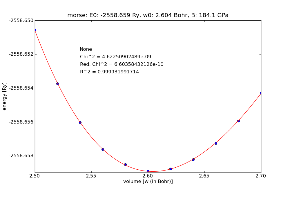
WS-radius vs. energy curve of fcc CoCrFeMnNi.

WS-radius vs. magnetic moments of fcc CoCrFeMnNi.